How to create a Pivot Table report

Pivot tables (also known as a "crosstab", "cross-tabulation", "matrix") allow you to summarize and analyze data in terms of groups; with pivot tables you can perform comparisons, explore trends and get answers on questions like "how many", "what is happened" and "why". Pivot tables remain most useful way to explore data both by non-IT users and professionals.

With SeekTable you can create pivot tables just in a few clicks:

1. Connect to your data: upload a CSV file or a setup database connection.
2. Add a new report: click on "Create Report" from cube, or choose "+" next to cube's name in the left menu.
   
3. Keep "Report Type" option at "Pivot table"
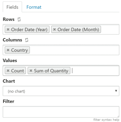
4. Choose grouping criteria: what columns to use for "Rows" and/or "Columns".
   Hold CTRL to select multiple items at once.
5. Choose a measure (aggregate function) to display in the pivot table: this may be count of rows, sum or average of the column. SeekTable will calculate aggregates for each row x column intersection. You can choose several measures at once.
6. Click on "Apply"

→

Sort Pivot Table

You can order table rows and columns in the following ways:

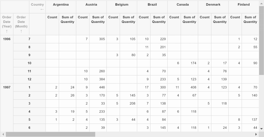
• By labels: order by values of the columns that are selected for "Rows" or "Columns". This is default sort option. To change order direction just click on the appropriate header at the top-left corner of the table:
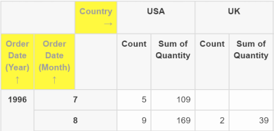
  • ← indicates A-Z order (ascending)
  • → indicates Z-A order (descending)
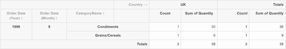
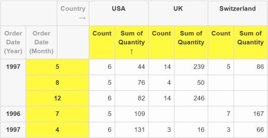• By values: order by the table's row (or column) values - that are calculatation results of the measure. To sort by a concrete row or column values click on the last grouping level label (or measure's name).
  • It is possible to keep order of groups by labels, and order by values only items in the last grouping level by checking "Sort by value last group only" option ("Format" tab).
  • Both rows and columns may be ordered by values if at least one axis is ordered by totals.

Filter pivot table

You can exclude some rows or columns (or show only concrete rows/columns) with a simple keyword-based Filter:

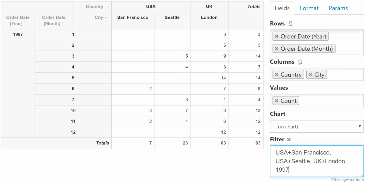
• Keywords for the same axis (rows or columns) are combined with OR. To force AND use + to combine conditions: year=2023+month=Jan
• To specify a keyword for concrete dimension's use dimension_keyword: prefix, for example: country:USA. For exact matches use = comparison: country=USA
• To match a phrase use quotes: name:"John Smith"
• To exclude matched items use - prefix, for example: -Venezuela.
• Show only top-N (or bottom-N) items in dimension's groups: country:top(5) or country:"top(5, 1)" (where "1" is a zero-based index of measure in report's Values). This filter works in the same way as Excel's PivotTable "Values Filter → Top-10" function.
• It is possible to filter pivot table by values: >5 (if a report has only one measure in Values) or sum>5 (to filter by measure that matches "sum").

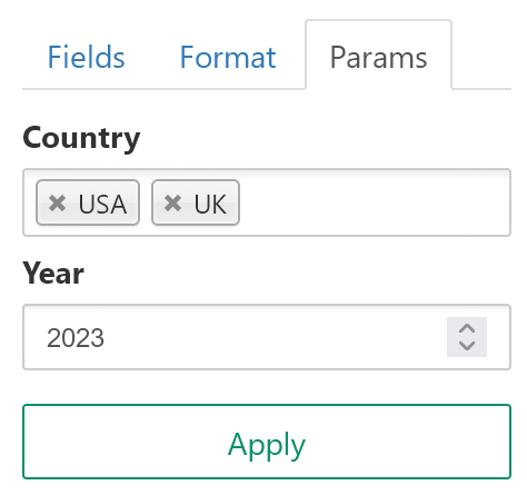
Another way to filter report's data are report parameters. Unlike table's "Filter" these parameters are always applied on a data source level; for instance, for SQL-based cubes these report parameters are converted to query's WHERE conditions. With report parameters it is possible to filter by dataset's columns that are not used in the report.

Report parameters may be configured only explicitly in the cube configuration form; please check your data source type help page for guidance. Params tab appears when at least one report parameter is configured for the cube.

Cells Formatting

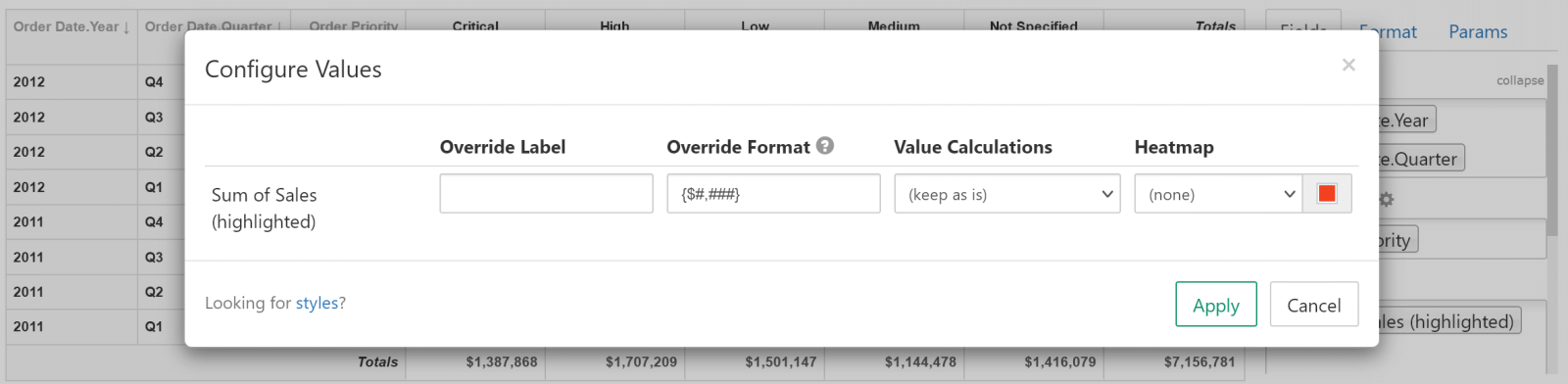
You can specify custom format for dimension's labels (table's rows & columns headers) and measures (cells with values) in this way:

1. Click on "gear" icon near Rows, Columns, Values.
2. Specify a custom format for an appropriate item with this pattern:

   <prefix> {value_format_specifier} <suffix>

   where value_format_specifier can be:

   # → display only integer part
   $#.## → display numbers as "$50.01" (empty if zero)
   $0.00 → display numbers as "$50.01" ("$0.00" if zero)
   yyyy-MM-dd → display dates as 2019-07-15
   MMM → format a month number (1-12) as a short month name (Jan, Feb etc)
   MMMM → format a month number (1-12) as a full month name (January, February etc)
   ddd → format a day-of-week number (0-6) as a short day-of-week name (Mon, Tue etc)
   dddd → format a day-of-week number (0-6) as a full day-of-week name (Monday, Tuesday etc)
   0.#|k → if number>1000 shorten it with "k" suffix
   0,.0# → show number in thousands (value divided by 1000)
   0.#|kMB → shorten large number with an appropriate "k"/"M"/"B" suffix
   ifempty=STR → if value is empty or null show "STR"
   

   For numbers formatting meaning of #, 0, ., , is the same as in Excel. For complete reference on format syntax see .NET String.Format documentation.
3. Also in this dialog you can specify custom labels if needed.

Drill Down

SeekTable offers great data exploration capabilities with a drill-down function: you can click on any pivot table cell with value and get more detailed view for this concrete group:

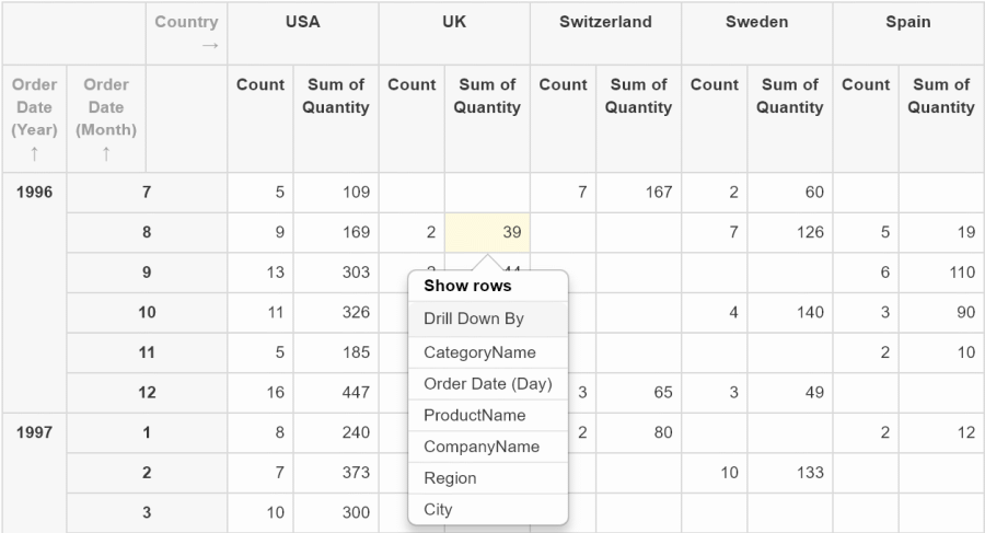
Cell's drill-down menu gives you 2 alternatives:

• Show rows: opens 'flat table' report pre-configured to display records of this group. Use browser's "Back" to return to the original pivot table. You can open this view in a new tab if you like (this is normal link).
  NOTE: "Show rows" option is not available if your pivot table uses expression-type dimensions or dimensions that are not allowed for 'flat table' report type.
• Drill down by dimension: you can choose which dimension to use to get more detailed view of the group. As result this dimension will be added to rows (or columns) and "Filter" will be changed to limit pivot table by the rows/columns that correspond to the group:

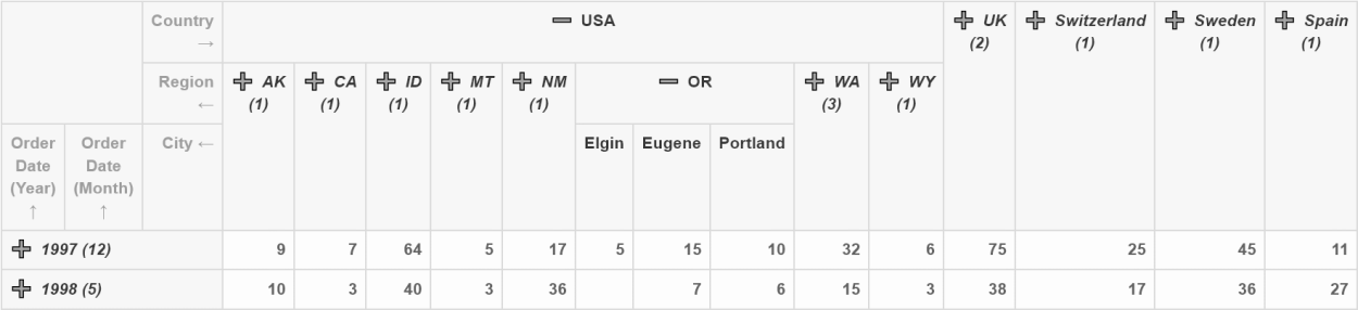
If you like Excel-like drill down by hierarchy with groups expand/collapse this is also possible:

• choose dimensions that you want to use as hierarchy for rows and/or columns. Hiearchy for dates might be: "Year", "Month", "Day". For location this could be "Country", "State", "City" and so on.
• Check Enable expand/collapse ("Format" tab) to activate this mode, or simply click on "collapse" link near "Rows" or "Columns".
• Click on "+" and "-" to expand/collapse individual groups:

SeekTable supports pagination for collapsed pivot tables. To show all rows and/or columns you may specify explicit Limits ("Format" tab) in the same way as for non-collapsed pivots.

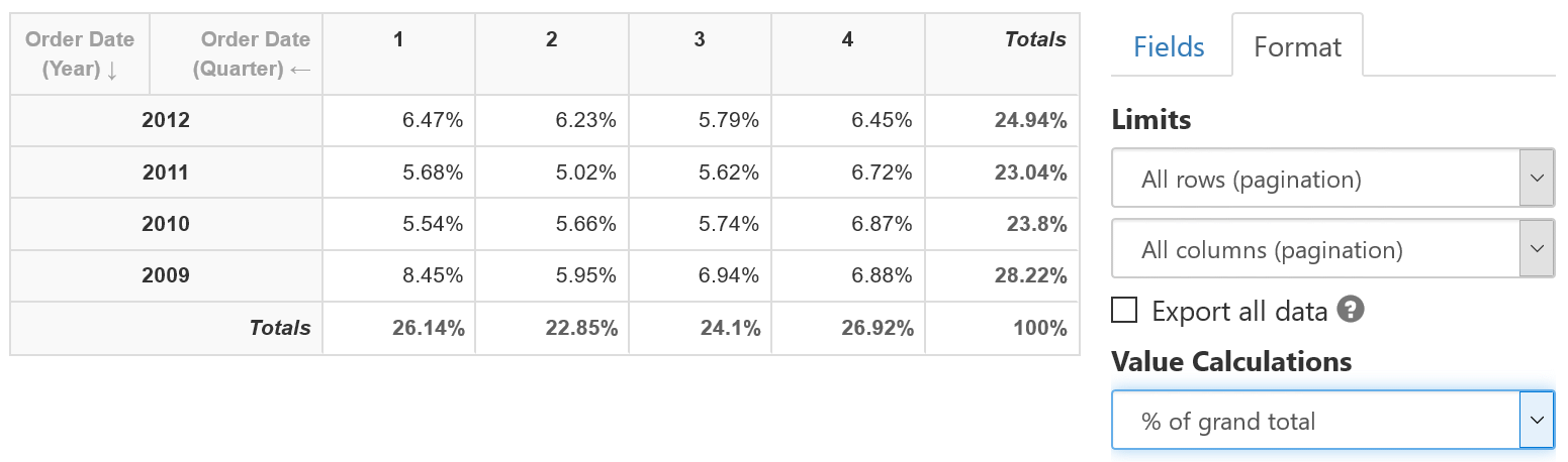
Pivot Table Percentage

To show values as percentages such as "% of Grand Total" or "% of Row Total" or "% of Column Total":

1. open Format tab
2. in the Value Calculations dropdown choose an appropriate option:

Data bars

It is possible to display percentage calculation as data bars that can improve table's readability a lot.

1. open Format tab
2. ensure that in Value Calculations a percentage option is selected ("% of ...")
3. Data bars checkbox appear to control whether percents should be visualized as data bars.
4. Click on "gear" icon to configure options like color, display value and which cells should have bars (all, values and subtotals, or only values).

Data bars are present PDF and Excel exports.

Pivot Table Top 10 show only top N (last N) rows and/or columns

To show only first top 10 (or top 5, top 100 etc) results in a pivot table:

1. open Format tab
2. use appropriate Limits dropdown to apply a top-N filter for either rows or columns or both:
3. click on Apply

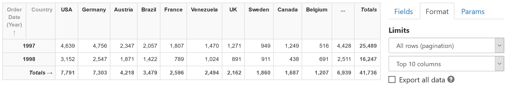
All results that are beyond the limit are included into special "..." group. To hide this group you can uncheck Show "..." group in case of limit .

Alternatively, it is possible to apply "top-N" filter per grouped items separately in the same way as in Excel PivotTables. This is useful when you want to show, say, top-10 'best' product categories and then top-5 'best' products in each category; to do that it is enough to add this into Filter textbox: category:top(10), product:top(5) (assuming that the report has "category" and "product" dimensions on the same axis).

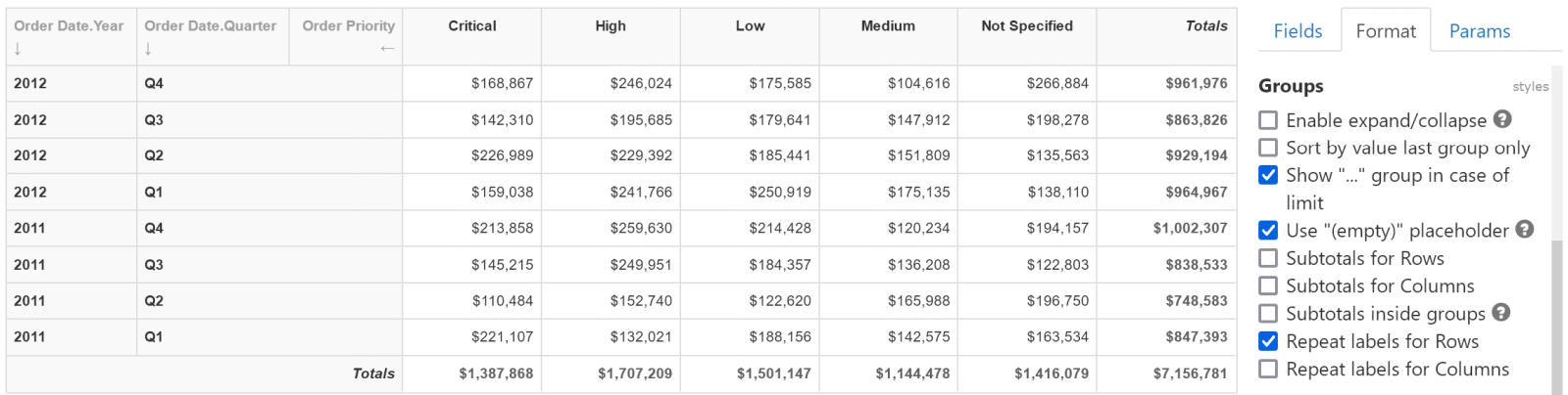
Repeat Labels in a Pivot Table

It is possible to repeat labels of grouped items in the same way as you can do that in Excel PivotTable:

1. open Format tab
2. check either Repeat labels for Rows or Repeat labels for Columns (or both)
3. click on Apply

Exports

SeekTable can export pivot tables to all popular export formats: CSV, PDF, Excel, HTML. For PDF/Excel exports the layout is identical to a web view. In Excel exports SeekTable tries to preserve all formatting (excluding custom HTML; colors/links for cells are preserved in Excel export). If SeekTable's pivot report has a chart it is also exported as an Excel Chart in a separate worksheet (this is a rather unique capability).

Additionally, a special "Excel PivotTable" export is possible; it works in this way:

• report's aggregated (summary) dataset is exported to "Report Data" worksheet
• in the main "Report" worksheet an Excel's PivotTable is created automatically (based on the summary data from the "Report Data" worksheet). SeekTable tries to pre-configure it similar to report's web view; however in Excel some calculations work differently (in particular, "differences" and "percentages") + for SeekTable-calculated measures (Type=Expression) totals may show wrong numbers.

By default exports include only data that you see in a web view (current page only, if pagination is used). If you want to export all rows/columns you may check Export all data option, and in this case export will include as much rows as possible (up to 50,000 on cloud SeekTable; this limit can be increased on self-hosted SeekTable).

Limitations

• Max number of value cells in the table (rows x columns): 1,000,000
  This limit can be increased in a self-hosted SeekTable.
• Max number of rows (unpaginated, non-collapsed): 50,000
• Max number of columns (unpaginated, non-collapsed): 1,000
• Number ranges depending on the measure type:

  Count	from 0 to 4294967295 (uint32)
  Sum, Average, Quantile	(+/-) 79,228,162,514,264,337,593,543,950,335 (up to 29 significant decimal digits) or (from -296 to 296) / 10(0 to 28) (.NET System.Decimal)
  Variance	from -1.79769313486232e308 to 1.79769313486232e308 (.NET System.Double)
  FirstValue, Min, Max	Value's datatype returned from a data source is preserved.